Intended for healthcare professionals
12. Survival analysis
Survival analysis is concerned with studying the time between entry to a study and a subsequent event. Originally the analysis was concerned with time from treatment until death, hence the name, but survival analysis is applicable to many areas as well as mortality. Recent examples include time to discontinuation of a contraceptive, maximum dose of bronchoconstrictor required to reduce a patient’s lung function to 80% of baseline, time taken to exercise to maximum tolerance, time that a transdermal patch can be left in place, time for a leg fracture to heal.
When the outcome of a study is the time between one event and another, a number of problems can occur.
- The times are most unlikely to be Normally distributed.
- We cannot afford to wait until events have happened to all the subjects, for example until all are dead. Some patients might have left the study early – they are lost to follow up. Thus the only information we have about some patients is that they were still alive at the last follow up. These are termed censored observations
Kaplan-Meier survival curve
We look at the data using a Kaplan-Meier survival curve. Suppose that the survival times, including censored observations, after entry into the study (ordered by increasing duration) of a group of n subjects are  The proportion of subjects, S(t), surviving beyond any follow up time (
 ) is estimated by
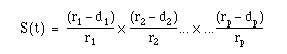 where
where 
= 0.
Method
Order the survival time by increasing duration starting with the shortest one. At each event (i) work out the number alive immediately before the event (r i). Before the first event all the patients are alive and so S(t) = 1. If we denote the start of the study as  , where = 0, then we have S
  = 1. We can now calculate the survival times
  , for each value of i from 1 to n by means of the following recurrence formula.
Given the number of events (deaths),  , at time and the number alive,
 , just before calculate
We do this only for the events and not for censored observations. The survival curve is unchanged at the time of a censored observation, but at the next event after the censored observation the number of people “at risk” is reduced by the number censored between the two events.
Example of calculation of survival curve
Mclllmurray and Turkie (2) describe a clinical trial of 69 patients for the treatment of Dukes’ C colorectal cancer. The data for the two treatments, linoleic acid or control are given in Table 12.1 (3).
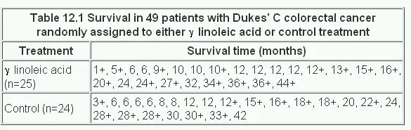
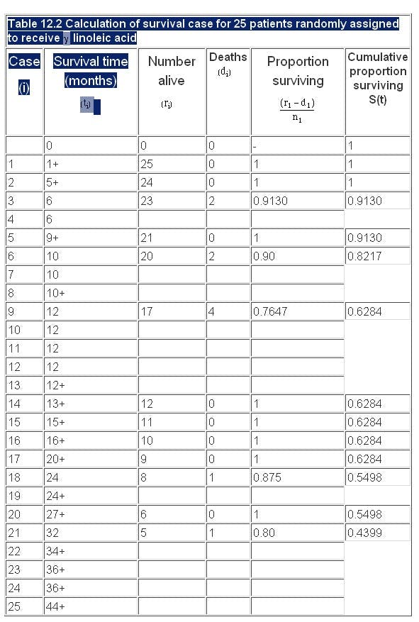
The calculation of the Kaplan-Meier survival curve for the 25 patients randomly assigned to receive 7 linoleic acid is described in Table 12.2 . The + sign indicates censored data. Until 6 months after treatment, there are no deaths, 50 S(t) 1. The effect of the censoring is to remove from the alive group those that are censored. At time 6 months two subjects have been censored and so the number alive just before 6 months is 23. There are two deaths at 6 months.
Thus,
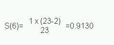
We now reduce the number alive (“at risk”) by two. The censored event at 9 months reduces the “at risk” set to 20. At 10 months there are two deaths, so the proportion surviving is 18/20 = 0.90 and the cumulative proportion surviving is 0.913 x 0.90 = 0.8217. The cumulative survival is conveniently stored in the memory of a calculator. As one can see the effect of the censored observations is to reduce the number at risk without affecting the survival curve S(t).
Finally we plot the survival curve, as shown in . The censored observations are shown as ticks on the line.
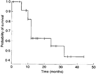
Figure 12.1 Survival curve of 25 patients with Dukes’ C colorectal cancer treated with linoleic acid.
Log rank test
To compare two survival curves produced from two groups A and B we use the rather curiously named log rank test,1 so called because it can be shown to be related to a test that uses the logarithms of the ranks of the data.
The assumptions used in this test are:
- That the survival times are ordinal or continuous.
- That the risk of an event in one group relative to the other does not change with time. Thus if linoleic acid reduces the risk of death in patients with colorectal cancer, then this risk reduction does not change with time (the so called proportional hazards assumption ).
We first order the data for the two groups combined, as shown in Table 12.3 . As for the Kaplan-Meier survival curve, we now consider each event in turn, starting at time t = 0.
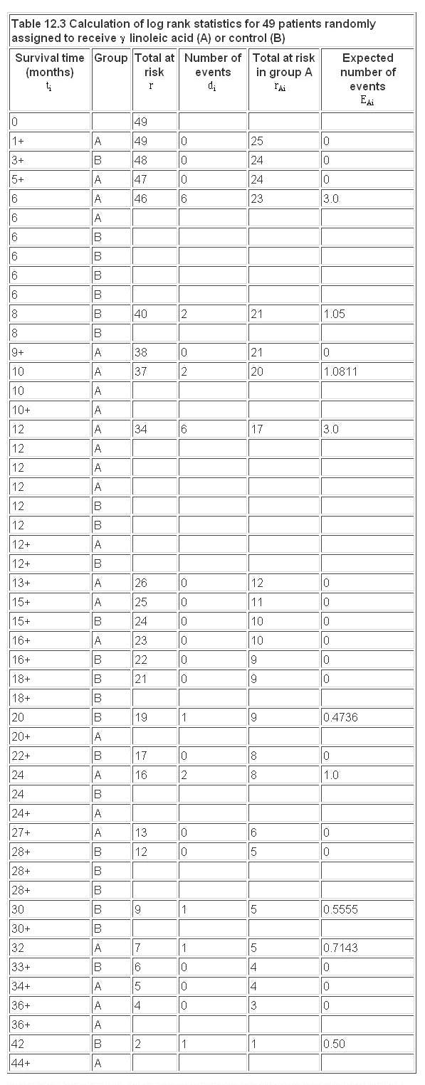
At each event (death) at time we consider the total number alive and the total number still alive in group A  up to that point. If we had a total of events at time then, under the null hypothesis, we consider what proportion of these would have been expected in group A. Clearly the more people at risk in one group the more deaths (under the null hypothesis) we would expect.
The effect of the censored observations is to reduce the numbers at risk, but they do not contribute to the expected numbers.
Further methods
In the same way that multiple regression is an extension of linear regression, an extension of the log rank test includes, for example, allowance for prognostic factors. This was developed by DR Cox, and so is called Cox regression. It is beyond the scope of this book, but is described elsewhere.(4, 5)
Common questions
Do I need to test for a constant relative risk before doing the log rank test?
This is a similar problem to testing for Normality for a t test. The log rank test is quite “robust” against departures from proportional hazards, but care should be taken. If the Kaplan-Meier survival curves cross then this is clear departure from proportional hazards, and the log rank test should not be used. This can happen, for example, in a two drug trial for cancer, if one drug is very toxic initially but produces more long term cures. In this case there is no simple answer to the question “is one drug better than the other?”, because the answer depends on the time scale.
If I don’t have any censored observations, do I need to use survival analysis?
Not necessarily, you could use a rank test such as the Mann-Whitney U test, but the survival method would yield an estimate of risk, which is often required, and lends itself to a useful way of displaying the data.
References
- Peto R, Pike MC, Armitage P et al . Design and analysis of randomized clinical trials requiring prolonged observation of each patient: II. Analysis and examples. Br J Cancer l977; 35 :l-39.
- McIllmurray MB, Turkie W. Controlled trial of linoleic acid in Dukes’ C colorectal cancer. BMJ 1987; 294 :1260, 295 :475.
- Gardner MJ, Altman DG (Eds). In: Statistics with Confidence, Confidence Intervals and Statistical Guidelines . London: BMJ Publishing Group, 1989; Chapter 7.
- Armitage P, Berry G. In: Statistical Methods in Medical Practice . Oxford: Blackwell Scientific Publications, 1994:477-81.
- Altman DG. Practical Statistics for Medical Research .. London: Chapman & Hall, 1991.
Exercises
12.1 Twenty patients, ten of normal weight and ten severely overweight underwent an exercise stress test, in which they had to lift a progressively increasing load for up to 12 minutes, but they were allowed to stop earlier if they could do no more. On two occasions the equipment failed before 12 minutes. The times (in minutes) achieved were:
Normal weight: 4, 10, 12*, 2, 8, 12*, 8**, 6, 9, 12*
Overweight: 7**, 5, 11, 6, 3, 9, 4, 1, 7, 12*
*Reached end of test; **equipment failure. (I am grateful to C Osmond for these data). What are the observed and expected values? What is the value of the log rank test to compare these groups?
12.2 What is the risk of stopping in the normal weight group compared with the overweight group, and a 95% confidence interval?