8. The Chi squared tests

The distribution of a categorical variable in a sample often needs to be compared with the distribution of a categorical variable in another sample. For example, over a period of 2 years a psychiatrist has classified by socioeconomic class the women aged 20-64 admitted to her unit suffering from self poisoning sample A. At the same time she has likewise classified the women of similar age admitted to a gastroenterological unit in the same hospital sample B. She has employed the Registrar General’s five socioeconomic classes, and generally classified the women by reference to their father’s or husband’s occupation. The results are set out in table 8.1.

The psychiatrist wants to investigate whether the distribution of the patients by social class differed in these two units. She therefore erects the null hypothesis that there is no difference between the two distributions. This is what is tested by the chi squared (χ²) test (pronounced with a hard ch as in “sky”). By default, all χ² tests are two sided.

It is important to emphasise here that χ² tests may be carried out for this purpose only on the actual numbers of occurrences, not on percentages, proportions, means of observations, or other derived statistics. Note, we distinguish here the Greek (χ²) for the test and the distribution and the Roman (x²) for the calculated statistic, which is what is obtained from the test.

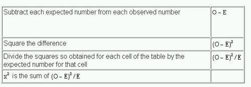
The χ² test is carried out in the following steps:

For each observed number (0) in the table find an “expected” number (E); this procedure is discussed below.

To calculate the expected number for each cell of the table consider the null hypothesis, which in this case is that the numbers in each cell are proportionately the same in sample A as they are in sample B. We therefore construct a parallel table in which the proportions are exactly the same for both samples. This has been done in columns (2) and (3) of table 8.2 . The proportions are obtained from the totals column in table 8.1 and are applied to the totals row. For instance, in table 8.2 , column (2), 11.80 = (22/289) x 155; 24.67 = (46/289) x 155; in column (3) 10.20 = (22/289) x 134; 21.33 = (46/289) x 134 and so on.

Thus by simple proportions from the totals we find an expected number to match each observed number. The sum of the expected numbers for each sample must equal the sum of the observed numbers for each sample, which is a useful check. We now subtract each expected number from its corresponding observed number.

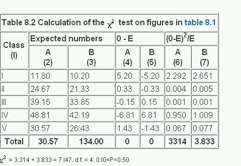
The results are given in columns (4) and (5) of table 8.2 . Here two points may be noted.

Again these are useful checks.

The figures in columns (4) and (5) are then each squared and divided by the corresponding expected numbers in columns (2) and (3). The results are given in columns (6) and (7). Finally these results, (O-E)²/E are added. The sum of them is x²

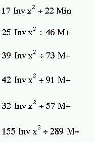
A helpful technical procedure in calculating the expected numbers may be noted here. Most electronic calculators allow successive multiplication by a constant multiplier by a short cut of some kind. To calculate the expected numbers a constant multiplier for each sample is obtained by dividing the total of the sample by the grand total for both samples. In table 8.1 for sample A this is 155/289 = 0.5363. This fraction is then successively multiplied by 22, 46, 73, 91, and 57. For sample B the fraction is 134/289 = 0.4636. This too is successively multiplied by 22, 46, 73, 91, and 57.

The results are shown in table 8.2 , columns (2) and (3).

Having obtained a value for we look up in a table of χ² distribution the probability attached to it (Appendix Table C.pdf ). Just as with the t table, we must enter this table at a certain number of degrees of freedom. To ascertain these requires some care.

When a comparison is made between one sample and another, as in table 8.1 , a simple rule is that the degrees of freedom equal (number of columns minus one) x (number of rows minus one) (not counting the row and column containing the totals). For the data in table 8.1 this gives (2 – 1) x (5 – 1) = 4. Another way of looking at this is to ask for the minimum number of figures that must be supplied in table 8.1 , in addition to all the totals, to allow us to complete the whole table. Four numbers disposed anyhow in samples A and B provided they are in separate rows will suffice.

Entering Table C at four degrees of freedom and reading along the row we find that the value of x²(7.147) lies between 3.357 and 7.779. The corresponding probability is: 0.10

The above method of calculating x² illustrates the nature of the statistic clearly and is often used in practice. A quicker method, similar to the quick method for calculating the standard deviation, is particularly suitable for use with electronic calculators.(1)

The data are set out as in table 8.1 . Take the left hand column of figures (Sample A) and call each observation a. Their total, which is 155, is then .

Let p = the proportion formed when each observation a is divided by the corresponding figure in the total column. Thus here p in turn equals 17/22, 25/46… 32/57.

Let = the proportion formed when the total of the observations in the left hand column, , is divided by the total of all the observations.

Here = 155/289. Let = 1 – , which is the same as 134/289.

Then

Working with the figures in table 8.1, we use this formula on an electronic calculator (Casio fx-350) in the following way:

Withdraw result from memory on to display screen

MR (1.7769764)

We now have to divide this by Here = 155/289 and = 134/289.

This gives us x²= 7.146.

The calculation naturally gives the same result if the figures for sample B are used instead of those for sample A. Owing to rounding off of the numbers the two methods for calculating x² may lead to trivially different results.

A special form of the χ² test is particularly common in practice and quick to calculate. It is applicable when the results of an investigation can be set out in a “fourfold table” or “2 x 2 contingency table”.

For example, the practitioner whose data we displayed in believed that the wives of the printers and farmers should be encouraged to breast feed their babies. She has records for her practice going back over 10 years, in which she has noted whether the mother breast fed the baby for at least 3 months or not, and these records show whether the husband was a printer or a sheep farmer (or some other occupation less well represented in her practice). The figures from her records are set out in table 8.3

The disparity seems considerable, for, although 28% of the printers’ wives breast fed their babies for three months or more, as many as 45% of the farmers’ wives did so. What is its significance?

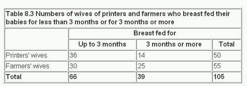
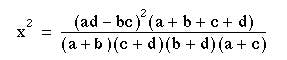
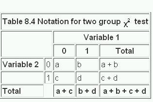
The null hypothesis is set up that there is no difference between printers’ wives and farmers’ wives in the period for which they breast fed their babies. The χ² test on a fourfold table may be carried out by a formula that provides a short cut to the conclusion. If a, b, c, and d are the numbers in the cells of the fourfold table as shown in table 8.4 (in this case Variable 1 is breast feeding ( < 3 months 0, 3 months 1) and Variable 2 is husband’s occupation (Printer (0) or Farmer (1)), x²is calculated from the following formula:

With a fourfold table there is one degree of freedom in accordance with the rule given earlier.

As many electronic calculators have a capacity limited to eight digits, it is advisable not to do all the multiplication or all the division in one series of operations, lest the number become too big for the display.

Multiply a by d and store in memory

Multiply b by c and subtract from memory

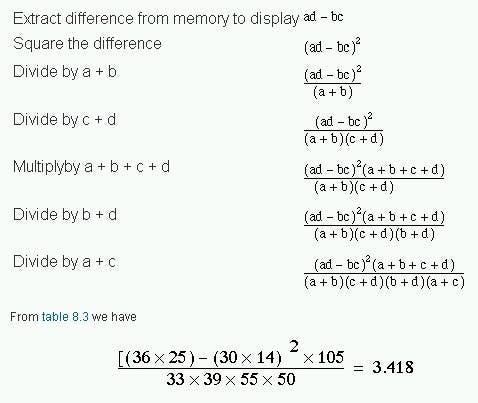
Entering the χ² table with one degree of freedom we read along the row and find that 3.418 lies between 2.706 and 3.84 1. Therefore 0.05

We now calculate a confidence interval of the differences between the two proportions, as described in Chapter 6 In this case we use the standard error based on the observed data, not the null hypothesis. We could calculate the confidence interval on either the rows or the columns and it is important that we compare proportions of the outcome variable, that is, breast feeding.

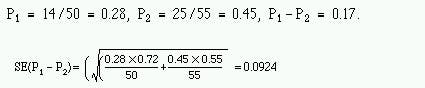
The 95% confidence interval is

0.17 – 1.96 x 0.0924 to 0.17 + 1.96 x 0.0924 = -0.011 to 0.351

Thus the 95% confidence interval is wide, and includes zero, as one might expect because the χ² test was not significant at the 5% level.

It can be shown mathematically that if χ is a Normally distributed variable, mean zero and variance 1, then x² has a χ² distribution with one degree of freedom. The converse also holds true and we can use this fact to improve the precision of our P values. In the above example we have = 3.418, with one degree of freedom. Thus X = 1.85, and from we find P to be about 0.065. However, we do need the tables for more than one degree of freedom.

When the numbers in a 2 x 2 contingency table are small, the χ² approximation becomes poor. The following recommendations may be regarded as a sound guide. (2) In fourfold tables a χ² test is inappropriate if the total of the table is less than 20, or if the total lies between 20 and 40 and the smallest expected (not observed) value is less than 5; in contingency tables with more than one degree of freedom it is inappropriate if more than about one fifth of the cells have expected values less than 5 or any cell an expected value of less than 1. An alternative to the χ² test for fourfold tables is known as Fisher’s Exact test and is described in Chapter 9

When the values in a fourfold table are fairly small a “correction for continuity” known as the “Yates’ correction” may be applied (3). Although there is no precise rule defining the circumstances in which to use Yates’ correction, a common practice is to incorporate it into χ² calculations on tables with a total of under 100 or with any cell containing a value less than 10. The χ² test on a fourfold table is then modified as follows:

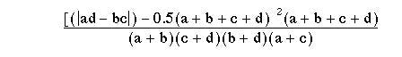
The vertical bars on either side of ad – bc mean that the smaller of those two products is taken from the larger. Half the total of the four values is then subtracted from that the difference to provide Yates’ correction. The effect of the correction is to reduce the value of x².

Applying it to the figures in table 8.3 gives the following result:

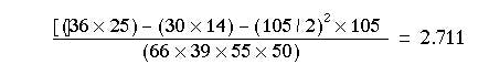
In this case x²=2.711 falls within the same range of P values as the x²= 3.418 we got without Yates’ correction (0.05

Earlier in this chapter we compared two samples by the χ² test to answer the question “Are the distributions of the members of these two samples between five classes significantly different?” Another way of putting this is to ask “Are the relative proportions of the two samples the same in each class?”

For example, an industrial medical officer of a large factory wants to immunise the employees against influenza. Five vaccines of various types based on the current viruses are available, but nobody knows which is preferable. From the work force 1350 employees agree to be immunised with one of the vaccines in the first week of December, 50 the medical officer divides the total into five approximately equal groups. Disparities occur between their total numbers owing to the layout of the factory complex. In the first week of the following March he examines the records he has been keeping to see how many employees got influenza and how many did not. These records are classified by the type of vaccine used ( table 8.5 ).

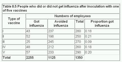
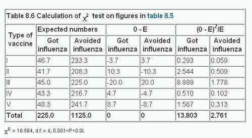
In table 8.6 the figures are analysed by the χ² test. For this we have to determine the expected values. The null hypothesis is that there is no difference between vaccines in their efficacy against influenza. We therefore assume that the proportion of employees contracting influenza is the same for each vaccine as it is for all combined. This proportion is derived from the total who got influenza, and is 225/1350. To find the expected number in each vaccine group who would contract the disease we multiply the actual numbers in the Total column of table 8.5 by this proportion. Thus 280 x (225/1350) = 46.7; 250 x (225/1350) = 41.7; and so on. Likewise the proportion who did not get influenza is 1125/1350.

The expected numbers of those who would avoid the disease are calculated in the same way from the totals in table 8.5, so that 280 x (1125/1350) = 233.3; 250 x (1250/1350) = 208.3; and so on.

The procedure is thus the same as shown in table 8.1 and table 8.2 .

The calculations made in table 8.6 show that χ² with four degrees of freedom is 16.564, and 0.001

Inspection of table 8.6 shows that the largest contribution to the total x² comes from the figures for vaccine III. They are 8.889 and 1.778, which together equal 10.667. If this figure is subtracted from the total x², 16.564 – 10.667 – 5.897. This gives an approximate figure for x² for the remainder of the table with three degrees of freedom (by removing the vaccine III we have reduced the table to four rows and two columns). We then find that 0.1

But this is not quite the end of the story. Before concluding from these figures that vaccine III is superior to the others we ought to carry out a check on other possible explanations for the disparity. The process of randomisation in the choice of the persons to receive each of the vaccines should have balanced out any differences between the groups, but some may have remained by chance. The sort of questions worth examining now are: Were the people receiving vaccine III as likely to be exposed to infection as those receiving the other vaccines? Could they have had a higher level of immunity from previous infection? Were they of comparable socioeconomic status? Of similar age on average? Were the sexes comparably distributed? Although some of these characteristics could have been more or less balanced by stratified randomisation, it is as well to check that they have in fact been equalised before attributing the numeral discrepancy in the result to the potency of the vaccine.

Table 8.1 is a 5 x 2 table, because there are five socioeconomic classes and two samples. Socioeconomic groupings may be thought of as an example of an ordered categorical variable, as there are some outcomes (for example, mortality) in which it is sensible to state that (say) social class II is between social class I and social class III. The χ² test described at that stage did not make use of this information; if we had interchanged any of the rows the value of x² would have been exactly the same. Looking at the proportions p in table 8.1 we can see that there is no real ordering by social class in the proportions of self poisoning; social class V is between social classes I and II. However in many cases, when the outcome variable is an ordered categorical variable, a more powerful test can be devised which uses this information.

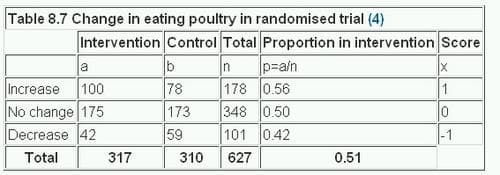
Consider a randomised controlled trial of health promotion in general practice to change people’s eating habits.(5) Table 8.7 gives the results from a review at 2 years, to look at the change in the proportion eating poultry.

If we give each category a score x the χ² test for trend is calculated in the following way:

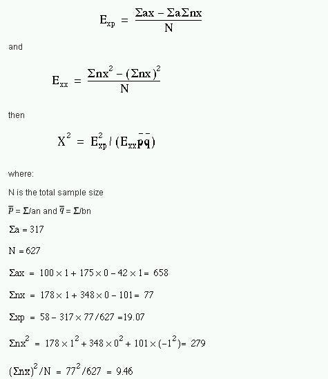
Thus

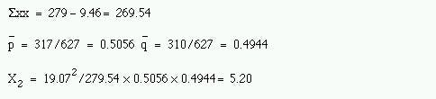
This has one degree of freedom because the linear scoring means that when one expected value is given all the others are fixed, and we find p = 0.02. The usual χ² test gives a value of = 5.51; d.f. = 2; 0.05

Note that this is another way of splitting the overall x² statistic. The overall x² will always be greater than the for trend, but because the latter uses only one degree of freedom, it is often associated with a smaller probability. Although one is often counselled not to decide on a statistical test after having looked at the data, it is obviously sensible to look at the proportions to see if they are plausibly monotonic (go steadily up or down) with the ordered variable, especially if the overall χ² test is nonsignificant.

Comparison of an observed and a theoretical distribution

In the cases so far discussed the observed values in one sample have been compared with the observed values in another. But sometimes we want to compare the observed values in one sample with a theoretical distribution.

For example, a geneticist has a breeding population of mice in his laboratory. Some are entirely white, some have a small patch of brown hairs on the skin, and others have a large patch. According to the genetic theory for the inheritance of these coloured patches of hair the population of mice should include 51.0% entirely white, 40.8% with a small brown patch, and 8.2% with a large brown patch. In fact, among the 784 mice in the laboratory 380 are entirely white, 330 have a small brown patch, and 74 have a large brown patch. Do the proportions differ from those expected?

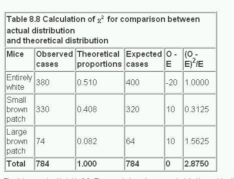
The data are set out in table 8.8 . The expected numbers are calculated by applying the theoretical proportions to the total, namely 0.510 x 784, 0.408 x 784, and 0.082 x 784. The degrees of freedom are calculated from the fact that the only constraint is that the total for the expected cases must equal the total for the observed cases, and so the degrees of freedom are the number of rows minus one. Thereafter the procedure is the same as in previous calculations of x². In this case it comes to 2.875. The x² table is entered at two degrees of freedom. We find that 0.2

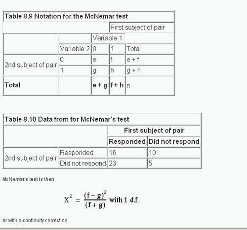
McNemar’s test for paired nominal data was described in , using a Normal approximation. In view of the relationship between the Normal distribution and the χ² distribution with one degree of freedom, we can recast the McNemar test as a variant of a χ² test. The results are often expressed as in table 8.9.

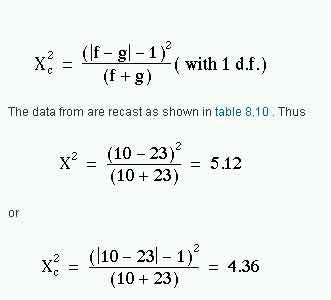
From appendix-table-c.pdf we find that for both χ² values 0.02

Extensions of the χ² test

If the outcome variable in a study is nominal, the χ² test can be extended to look at the effect of more than one input variable, for example to allow for confounding variables. This is most easily done using multiple logistic regression , a generalisation of multiple regression , which is described in Chapter 11. If the data are matched, then a further technique ( conditional logistic regression ) should be employed. This is described in advanced textbooks and will not be discussed further here.

I have matched data, but the matching criteria were very weak. Should I use McNemar’s test?

The general principle is that if the data are matched in any way, the analysis should take account of it. If the matching is weak then the matched analysis and the unmatched analysis should agree. In some cases when there are a large number of pairs with the same outcome, it would appear that the McNemar’s test is discarding a lot of information, and so is losing power. However, imagine we are trying to decide which of two high jumpers is the better. They each jump over a bar at a fixed height, and then the height is increased. It is only when one fails to jump a given height and the other succeeds that a winner can be announced. It does not matter how many jumps both have cleared.

8.1 In a trial of new drug against a standard drug for the treatment of depression the new drug caused some improvement in 56% of 73 patients and the standard drug some improvement in 41% of 70 patients. The results were assessed in five categories as follows:

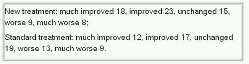
What is the value of x² which takes no account of the ordered value of data, what is the value of the x² test for trend, and the P value? How many degrees of freedom are there? What is the value of P in each case?

8.2 An outbreak of pediculosis capitis is being investigated in a girls’ school containing 291 pupils. Of 130 children who live in a nearby housing estate 18 were infested and of 161 who live elsewhere 37 were infested. What is the x² value of the difference, and what is its significance? Find the difference in infestation rates and a 95% confidence interval for the difference.

8.3 The 55 affected girls were divided at random into two groups of 29 and 26. The first group received a standard local application and the second group a new local application. The efficacy of each was measured by clearance of the infestation after one application. By this measure the standard application failed in ten cases and the new application in five. What is the χ² value of the difference (with Yates’ correction), and what is its significance? What is the difference in clearance rates and an approximate 95% confidence interval?

8.4 A general practitioner reviewed all patient notes in four practices for 1 year. Newly diagnosed cases of asthma were noted, and whether or not the case was referred to hospital. The following referrals were found (total cases in parentheses): practice A, 14 (103); practice B, 11 (92); practice C, 39 (166); practice D, 31 (221). What are the x² and P values for the distribution of the referrals in these practices? Do they suggest that any one practice has significantly more referrals than others?

References

- Snedecor GW, Cochran WG. In: Statistical Methods , 7th ed. Iowa: Iowa State University Press, 191,0:47.
- Cochran WG. Some methods for strengthening the common χ² tests. Biometrics 1956; l0 :4l7-5l.
- Yates F. Contingency tables involving small numbers and the χ² test. J Roy Stat Soc Suppl 1934; 1:217-3.
- Capples ME, McKnight A. Randomised controlled trial of health promotions in general practice for patients at high cardiovascular risk. BMJ l994;3O9:993-6.