2. Mean and standard deviation

 

The median is known as a measure of location; that is, it tells us where the data are. As stated in , we do not need to know all the exact values to calculate the median; if we made the smallest value even smaller or the largest value even larger, it would not change the value of the median. Thus the median does not use all the information in the data and so it can be shown to be less efficient than the mean or average, which does use all values of the data. To calculate the mean we add up the observed values and divide by the number of them. The total of the values obtained in Table 1.1 was 22.5 , which was divided by their number, 15, to give a mean of 1.5. This familiar process is
conveniently expressed by the following symbols:

(pronounced “x bar”) signifies the mean; x is each of the values of urinary lead; n is the number of these values; and σ , the Greek capital sigma (our “S”) denotes “sum of”. A major disadvantage of the mean is that it is sensitive to outlying points. For example, replacing 2.2 by 22 in Table 1.1 increases the mean to 2.82 , whereas the median will be unchanged.

As well as measures of location we need measures of how variable the data are. We met two of these measures, the range and interquartile range, in Chapter 1.

The range is an important measurement, for figures at the top and bottom of it denote the findings furthest removed from the generality. However, they do not give much indication of the spread of observations about the mean. This is where the standard deviation (SD) comes in.

The theoretical basis of the standard deviation is complex and need not trouble the ordinary user. We will discuss sampling and populations in Chapter 3. A practical point to note here is that, when the population from which the data arise have a distribution that is approximately “Normal” (or Gaussian), then the standard deviation provides a useful basis for interpreting the data in terms of probability.

The Normal distribution is represented by a family of curves defined uniquely by two parameters, which are the mean and the standard deviation of the population. The curves are always symmetrically bell shaped, but the extent to which the bell is compressed or flattened out depends on the standard deviation of the population. However, the mere fact that a curve is bell shaped does not mean that it represents a Normal distribution, because other distributions may have a similar sort of shape.

Many biological characteristics conform to a Normal distribution closely enough for it to be commonly used – for example, heights of adult men and women, blood pressures in a healthy population, random errors in many types of laboratory measurements and biochemical data. Figure 2.1 shows a Normal curve calculated from the diastolic blood pressures of 500 men, mean 82 mmHg, standard deviation 10 mmHg. The ranges representing [+-1SD, +12SD, and +-3SD] about the mean are marked. A more extensive set of values is given in Table A of the print edition.

Figure 2.1

The reason why the standard deviation is such a useful measure of the scatter of the observations is this: if the observations follow a Normal distribution, a range covered by one standard deviation above the mean and one standard deviation below it

includes about 68% of the observations; a range of two standard deviations above and two below () about 95% of the observations; and of three standard deviations above and three below () about 99.7% of the observations. Consequently, if we know the mean and standard deviation of a set of observations, we can obtain some useful information by simple arithmetic. By putting one, two, or three standard deviations above and below the mean we can estimate the ranges that would be expected to include about 68%, 95%, and 99.7% of the observations.

The standard deviation is a summary measure of the differences of each observation from the mean. If the differences themselves were added up, the positive would exactly balance the negative and so their sum would be zero. Consequently the squares of the differences are added. The sum of the squares is then divided by the number of observations minus oneto give the mean of the squares, and the square root is taken to bring the measurements back to the units we started with. (The division by the number of observations minus oneinstead of the number of observations itself to obtain the mean square is because “degrees of freedom” must be used. In these circumstances they are one less than the total. The theoretical justification for this need not trouble the user in practice.)

To gain an intuitive feel for degrees of freedom, consider choosing a chocolate from a box of n chocolates. Every time we come to choose a
chocolate we have a choice, until we come to the last one (normally one with a nut in it!), and then we have no choice. Thus we have n-1 choices, or “degrees of freedom”.

The calculation of the variance is illustrated in Table 2.1 with the 15 readings in the preliminary study of urinary lead concentrations (Table 1.2). The readings are set out in column (1). In column (2) the difference between each reading and the mean is recorded. The sum of the differences is 0. In column (3) the differences are squared, and the sum of those squares is given at the bottom of the column.

Table 2.1

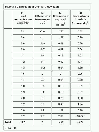
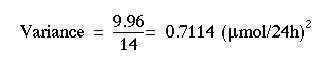
The sum of the squares of the differences (or deviations) from the mean, 9.96, is now divided by the total number of observation minus one, to give the variance.Thus,

In this case we find:

Finally, the square root of the variance provides the standard deviation:

from which we get
This procedure illustrates the structure of the standard deviation, in particular that the two extreme values 0.1 and 3.2 contribute most to the sum of the differences squared.

Most inexpensive calculators have procedures that enable one to calculate the mean and standard deviations directly, using the “SD” mode. For example, on modern Casio calculators one presses SHIFT and ‘.’ and a little “SD” symbol should appear on the display. On earlier Casios one presses INV and MODE , whereas on a Sharp 2nd F and Stat should be used. The data are stored via the M+ button. Thus, having set the calculator into the “SD” or “Stat” mode, from Table 2.1 we enter 0.1 M+ , 0.4 M+ , etc. When all the data are entered, we can check that the correct number of observations have been included by Shift and n, and “15” should be displayed. The mean is displayed by Shift and and the standard deviation by Shift and . Avoid pressing Shift and AC between these operations as this clears the statistical memory. There is another button on many calculators. This uses the divisor n rather than n – 1 in the calculation of the standard deviation. On a Sharp calculator is denoted , whereas is denoted s. These are the “population” values, and are derived assuming that an entire population is available or that interest focuses solely on the data in hand, and the results are not going to be generalised (see Chapter
3 for details of samples and populations). As this situation very rarely arises, should be used and ignored, although even for moderate sample sizes the difference is going to be small. Remember to return to normal mode before resuming calculations because many of the usual functions are not available in “Stat” mode. On a modern Casio this is Shift 0. On earlier Casios and on Sharps one repeats the sequence that call up the “Stat” mode. Some calculators stay in “Stat”
mode even when switched off.Mullee (1) provides advice on choosing and using a calculator. The calculator formulas use the relationship

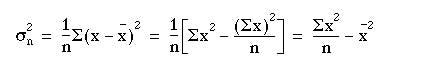
The right hand expression can be easily memorised by the expression mean of the squares minus the mean square”. The sample variance is obtained from

The above equation can be seen to be true in Table 2.1, where the sum of the square of the observations, , is given as 43.7l.

We thus obtain

the same value given for the total in column (3). Care should be taken because this formula involves subtracting two large numbers to get a small one, and can lead to incorrect results if the numbers are very large. For example, try finding the standard deviation of 100001, 100002, 100003 on a calculator. The correct answer is 1, but many calculators will give 0 because of rounding error. The solution is to subtract a large number from each of the observations (say 100000) and calculate the standard deviation on the remainders, namely 1, 2 and 3.

We can also calculate a standard deviation for discrete quantitative variables. For example, in addition to studying the lead concentration in the urine of 140 children, the paediatrician asked how often each of them had been examined by a doctor during the year. After collecting the information he tabulated the data shown in Table 2.2 columns (1) and (2). The mean is calculated by multiplying column (1) by column (2), adding the products, and dividing by the total number of observations. Table 2.2

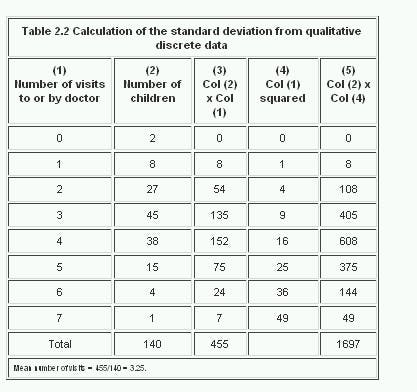
As we did for continuous data, to calculate the standard deviation we square each of the observations in turn. In this case the observation is the number of visits, but because we have several children in each class, shown in column (2), each squared number (column (4)), must be multiplied by the number of children. The sum of squares is given at the foot of column (5), namely 1697. We then use the calculator formula to find the variance: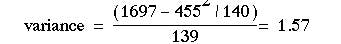and .Note that although the number of visits is not Normally distributed, the distribution is reasonably symmetrical about the mean. The approximate 95% range is given byThis excludes two children with no visits and
six children with six or more visits. Thus there are eight of 140 = 5.7% outside the theoretical 95% range.Note that it is common for discrete quantitative variables to have what is known as skeweddistributions, that is they are not symmetrical. One clue to lack of symmetry from derived statistics is when the mean and the median differ considerably. Another is when the standard deviation is of the same order of magnitude as the mean, but the observations must be non-negative. Sometimes a transformation will
convert a skewed distribution into a symmetrical one. When the data are counts, such as number of visits to a doctor, often the square root transformation will help, and if there are no zero or negative values a logarithmic transformation will render the distribution more symmetrical.

An anaesthetist measures the pain of a procedure using a 100 mm visual analogue scale on seven patients. The results are given in Table 2.3, together with the log etransformation (the ln button on a calculator). Table 2.3

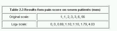The data are plotted in Figure 2.2, which shows that the outlier does not appear so extreme in the logged data. The mean and median are 10.29 and 2, respectively, for the original data, with a standard deviation of 20.22. Where the mean is bigger than the median, the distribution is positively skewed. For the logged data the mean and median are 1.24 and 1.10 respectively, indicating that the logged data have a more symmetrical distribution. Thus it would be better to analyse the logged transformed data
in statistical tests than using the original scale.Figure 2.2

In reporting these results, the median of the raw data would be given, but it should be explained that the statistical test wascarried out on the transformed data. Note that the median of the logged data is the same as the log of the median of the raw data – however, this is not true for the mean. The mean of the logged data is not necessarily equal to the log of the mean of the raw data.
The antilog (exp or on a calculator) of the mean of the logged data is known as the geometric mean,and is often a
better summary statistic than the mean for data from positively skewed distributions. For these data the geometric mean in 3.45 mm.

If repeated measurements are made of, say, blood pressure on an individual, these measurements are likely to vary. This is within subject, or intrasubject, variability and we can calculate a standard deviation of these observations. If the observations are close together in time, this standard deviation is often described as the measurement error.Measurements made on different subjects vary according to between subject, or intersubject, variability. If many observations were made on each individual, and the average taken, then we can assume that the intrasubject variability has been averaged out and the variation in the average values is due solely to the intersubject variability. Single observations on individuals clearly contain a mixture of intersubject and intrasubject variation. The coefficient of variation(CV%) is the intrasubject standard deviation divided by the mean, expressed as a percentage. It is often quoted as a measure of repeatability for biochemical assays, when an assay is carried out on several occasions on the same sample. It has the advantage of being independent of the units of measurement, but also numerous theoretical disadvantages. It is usually nonsensical to use the coefficient of variation as a measure of between subject variability.

When should I use the mean and when should I use the median to describe my
data?

It is a commonly held misapprehension that for Normally distributed data one uses the mean, and for non-Normally distributed data one uses the median. Alas this is not so: if the data are Normally distributed the mean and the median will be close; if the data are not Normally distributed then both the mean and the median may give useful information. Consider a variable that takes the value 1 for males and 0 for females. This is clearly not Normally distributed. However, the mean gives the proportion of males in the group, whereas the median merely tells us which group contained more than 50% of the people. Similarly, the mean from ordered categorical variables can be more useful than the median, if the ordered categories can be given meaningful scores. For example, a lecture might be rated as 1 (poor) to 5 (excellent). The usual statistic for summarising the result would be the mean. In the situation where there is a small group at one extreme of a distribution (for example, annual income) then the median will be more “representative” of the distribution. My data must have values greater than zero and yet the mean and standard deviation are about the same size. How does this happen? If data have a very skewed distribution, then the standard deviation will be grossly inflated, and is not a good measure of variability to use. As we have shown, occasionally a transformation of the data, such as a log transform, will render the distribution more symmetrical. Alternatively, quote the interquartile range.

1. Mullee M A. How to choose and use a calculator. In: How to do it 2.BMJ
Publishing Group, 1995:58-62.

In the campaign against smallpox a doctor inquired into the number of times 150 people aged 16 and over in an Ethiopian village had been vaccinated. He obtained the following figures: never, 12 people; once, 24; twice, 42; three times, 38; four times, 30; five times, 4. What is the mean number of times those people had been vaccinated and what is the standard deviation?Answer

Obtain the mean and standard deviation of the data in and an approximate
95% range.Answer

Which points are excluded from the range mean – 2SD to mean + 2SD? What
proportion of the data is excluded? Answers
Chapter 2 Q3.pdfAnswer