Intended for healthcare professionals

Home/About BMJ/Resources for readers/Publications/Statistics at square one/7. The t tests

7. The t tests

Previously we have considered how to test the null hypothesis that there is no difference between the mean of a sample and the population mean, and no difference between the means of two samples. We obtained the difference between the means by subtraction, and then divided this difference by the standard error of the difference. If the difference is 196 times its standard error, or more, it is likely to occur by chance with a frequency of only 1 in 20, or less.

With small samples, where more chance variation must be allowed for, these ratios are not entirely accurate because the uncertainty in estimating the standard error has been ignored. Some modification of the procedure of dividing the difference by its standard error is needed, and the technique to use is the t test. Its foundations were laid by WS Gosset, writing under the pseudonym “Student” so that it is sometimes known as Student’s t test. The procedure does not differ greatly from the one used for large samples, but is preferable when the number of observations is less than 60, and certainly when they amount to 30 or less.

The application of the t distribution to the following four types of problem will now be considered.

The calculation of a confidence interval for a sample mean.
The mean and standard deviation of a sample are calculated and a value is postulated for the mean of the population. How significantly does the sample mean differ from the postulated population mean?
The means and standard deviations of two samples are calculated. Could both samples have been taken from the same population?
Paired observations are made on two samples (or in succession on one sample). What is the significance of the difference between the means of the two sets of observations?

In each case the problem is essentially the same – namely, to establish multiples of standard errors to which probabilities can be attached. These multiples are the number of times a difference can be divided by its standard error. We have seen that with large samples 1.96 times the standard error has a probability of 5% or less, and 2.576 times the standard error a probability of 1% or less (Appendix table A ). With small samples these multiples are larger, and the smaller the sample the larger they become.

Confidence interval for the mean from a small sample

A rare congenital disease, Everley’s syndrome, generally causes a reduction in concentration of blood sodium. This is thought to provide a useful diagnostic sign as well as a clue to the efficacy of treatment. Little is known about the subject, but the director of a dermatological department in a London teaching hospital is known to be interested in the disease and has seen more cases than anyone else. Even so, he has seen only 18. The patients were all aged between 20 and 44.

The mean blood sodium concentration of these 18 cases was 115 mmol/l, with standard deviation of 12 mmol/l. Assuming that blood sodium concentration is Normally distributed what is the 95% confidence interval within which the mean of the total population of such cases may be expected to lie?

The data are set out as follows:

To find the 95% confidence interval above and below the mean we now have to find a multiple of the standard error. In large samples we have seen that the multiple is 1.96 (Chapter 4). For small samples we use the table of t given in Appendix Table B.pdf. As the sample becomes smaller t becomes larger for any particular level of probability. Conversely, as the sample becomes larger t becomes smaller and approaches the values given in table A, reaching them for infinitely large samples.

Since the size of the sample influences the value of t, the size of the sample is taken into account in relating the value of t to probabilities in the table. Some useful parts of the full t table appear in . The left hand column is headed d.f. for “degrees of freedom”. The use of these was noted in the calculation of the standard deviation (Chapter 2). In practice the degrees of freedom amount in these circumstances to one less than the number of observations in the sample. With these data we have 18 – 1 = 17 d.f. This is because only 17 observations plus the total number of observations are needed to specify the sample, the 18th being determined by subtraction.

To find the number by which we must multiply the standard error to give the 95% confidence interval we enter table B at 17 in the left hand column and read across to the column headed 0.05 to discover the number 2.110. The 95% confidence intervals of the mean are now set as follows:

Mean + 2.110 SE to Mean – 2.110 SE

which gives us:

115 – (2.110 x 283) to 115 + 2.110 x 2.83 or 109.03 to 120.97 mmol/l.

We may then say, with a 95% chance of being correct, that the range 109.03 to 120.97 mmol/l includes the population mean.

Likewise from Appendix Table B.pdf the 99% confidence interval of the mean is as follows:

Mean + 2.898 SE to Mean – 2.898 SE

which gives:

115 – (2.898 x 2.83) to 115 + (2.898 x 2.83) or 106.80 to 123.20 mmol/l.

Difference of sample mean from population mean (one sample t test)

Estimations of plasma calcium concentration in the 18 patients with Everley’s syndrome gave a mean of 3.2 mmol/l, with standard deviation 1.1. Previous experience from a number of investigations and published reports had shown that the mean was commonly close to 2.5 mmol/l in healthy people aged 20-44, the age range of the patients. Is the mean in these patients abnormally high?

We set the figures out as follows:

t difference between means divided by standard error of sample mean. Ignoring the sign of the t value, and entering table B at 17 degrees of freedom, we find that 2.69 comes between probability values of 0.02 and 0.01, in other words between 2% and 1% and so It is therefore unlikely that the sample with mean 3.2 came from the population with mean 2.5, and we may conclude that the sample mean is, at least statistically, unusually high. Whether it should be regarded clinically as abnormally high is something that needs to be considered separately by the physician in charge of that case.

Difference between means of two samples

Here we apply a modified procedure for finding the standard error of the difference between two means and testing the size of the difference by this standard error (see Chapter 5 for large samples). For large samples we used the standard deviation of each sample, computed separately, to calculate the standard error of the difference between the means. For small samples we calculate a combined standard deviation for the two samples.

The assumptions are:

that the data are quantitative and plausibly Normal
that the two samples come from distributions that may differ in their mean value, but not in the standard deviation
that the observations are independent of each other.
The third assumption is the most important. In general, repeated measurements on the same individual are not independent. If we had 20 leg ulcers on 15 patients, then we have only 15 independent observations.

The following example illustrates the procedure.

The addition of bran to the diet has been reported to benefit patients with diverticulosis. Several different bran preparations are available, and a clinician wants to test the efficacy of two of them on patients, since favourable claims have been made for each. Among the consequences of administering bran that requires testing is the transit time through the alimentary canal. Does it differ in the two groups of patients taking these two preparations?

The null hypothesis is that the two groups come from the same population. By random allocation the clinician selects two groups of patients aged 40-64 with diverticulosis of comparable severity. Sample 1 contains 15 patients who are given treatment A, and sample 2 contains 12 patients who are given treatment B. The transit times of food through the gut are measured by a standard technique with marked pellets and the results are recorded, in order of increasing time, in Table 7.1 .

Table 7.1

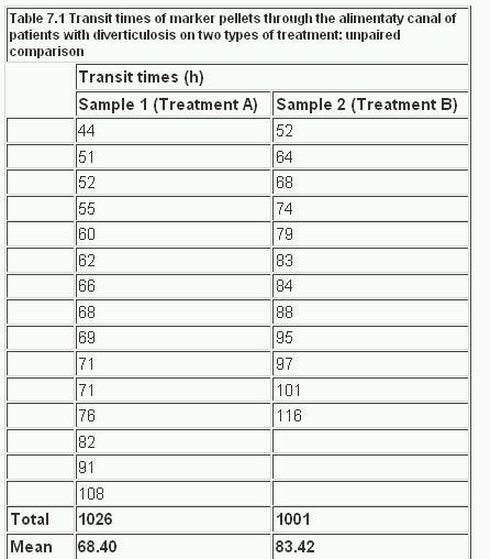
These data are shown in figure 7.1 . The assumption of approximate Normality and equality of variance are satisfied. The design suggests that the observations are indeed independent. Since it is possible for the difference in mean transit times for A-B to be positive or negative, we will employ a two sided test.

Figure 7.1

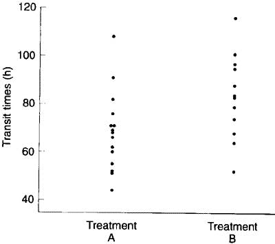
With treatment A the mean transit time was 68.40 h and with treatment B 83.42 h. What is the significance of the difference, 15.02h?

The procedure is as follows:

Obtain the standard deviation in sample 1:

Obtain the standard deviation in sample 2:

Multiply the square of the standard deviation of sample 1 by the degrees of freedom, which is the number of subjects minus one:

Repeat for sample 2

Add the two together and divide by the total degrees of freedom

The standard error of the difference between the means is

which can be written

When the difference between the means is divided by this standard error the result is t. Thus,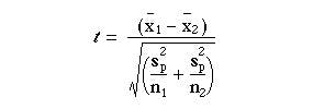

The table of the tdistribution Table B (appendix) which gives two sided P values is entered at degrees of freedom.

For the transit times of table 7.1,

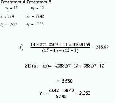shows that at 25 degrees of freedom (that is (15 – 1) + (12 – 1)), t= 2.282 lies between 2.060 and 2.485. Consequently, this degree of probability is smaller than the conventional level of 5%. The null hypothesis that there is no difference between the means is therefore somewhat unlikely.

A 95% confidence interval is given by

This becomes

83.42 – 68.40 2.06 x 6.582

15.02 – 13.56 to 15.02 + 13.56 or 1.46 to 18.58 h.

Unequal standard deviations

If the standard deviations in the two groups are markedly different, for example if the ratio of the larger to the smaller is greater than two, then one of the assumptions of the ttest (that the two samples come from populations with the same standard deviation) is unlikely to hold. An approximate test, due to Sattherwaite, and described by Armitage and Berry, (1)which allows for unequal standard deviations, is as follows.

Rather than use the pooled estimate of variance, compute

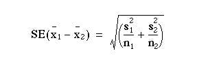This is analogous to calculating the standard error of the difference in two proportions under the alternative hypothesis as described in Chapter 6

We now compute

We then test this using a t statistic, in which the degrees of freedom are:

Although this may look very complicated, it can be evaluated very easily on a calculator without having to write down intermediate steps (see below). It can produce a degree of freedom which is not an integer, and so not available in the tables. In this case one should round to the nearest integer. Many statistical packages now carry out this test as the default, and to get the equal variances I statistic one has to specifically ask for it. The unequal variance t test tends to be less powerful than the usual t test if the variances are in fact the same, since it uses fewer assumptions. However, it should not be used indiscriminantly because, if the standard deviations are different, how can we interpret a nonsignificant difference in means, for example? Often a better strategy is to try a data transformation, such as taking logarithms as described in Chapter 2. Transformations that render distributions closer to Normality often also make the standard deviations similar. If a log transformation is successful use the usual t test on the logged data. Applying this method to the data of Table 7.1 , the calculator method (using a Casio fx-350) for calculating the standard error is:

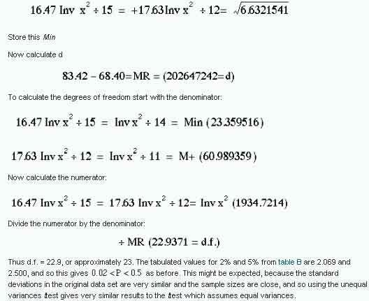
Difference between means of paired samples (paired t test).

When the effects of two alternative treatments or experiments are compared, for example in cross over trials, randomised trials in which randomisation is between matched pairs, or matched case control studies (see Chapter 13 ), it is sometimes possible to make comparisons in pairs. Matching controls for the matched variables, so can lead to a more powerful study.

The test is derived from the single sample t test, using the following assumptions.

The data are quantitative
The distribution of the differences (not the original data), is plausibly Normal.
The differences are independent of each other.

The first case to consider is when each member of the sample acts as his own control. Whether treatment A or treatment B is given first or second to each member of the sample should be determined by the use of the table of random numbers Table F (Appendix). In this way any effect of one treatment on the other, even indirectly through the patient’s attitude to treatment, for instance, can be minimised. Occasionally it is possible to give both treatments simultaneously, as in the treatment of a skin disease by applying a remedy to the skin on opposite sides of the body.

Let us use as an example the studies of bran in the treatment of diverticulosis discussed earlier. The clinician wonders whether transit time would be shorter if bran is given in the same dosage in three meals during the day (treatment A) or in one meal (treatment B). A random sample of patients with disease of comparable severity and aged 20-44 is chosen and the two treatments administered on two successive occasions, the order of the treatments also being determined from the table of random numbers. The alimentary transit times and the differences for each pair of treatments are set out in Table 7.2

Table 7.2

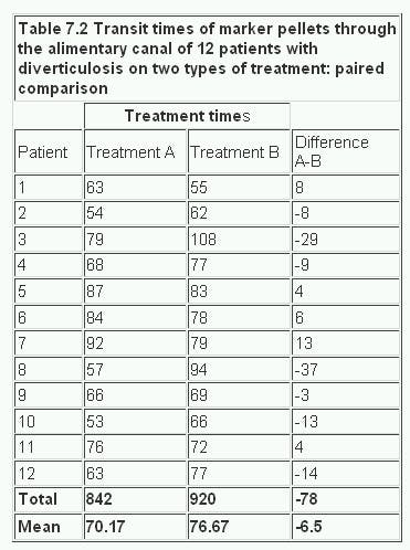
In calculating t on the paired observations we work with the difference, d, between the members of each pair. Our first task is to find the mean of the differences between the observations and then the standard error of the mean, proceeding as follows:

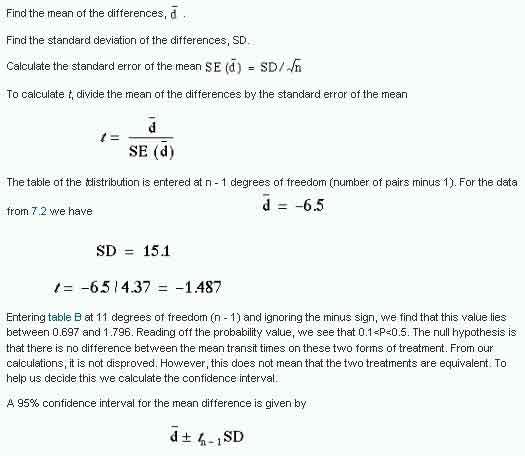
Entering Appendix Table B.pdf at 11 degrees of freedom (n – 1) and ignoring the minus sign, we find that this value lies between 0.697 and 1.796. Reading off the probability value, we see that 0.1

A 95% confidence interval for the mean difference is given by

In this case t 11 at P = 0.05 is 2.201 (table B) and so the 95% confidence interval is:

-6.5 – 2.201 x 4.37 to -6.5 + 2.201 x 4.37 h. or -16.1 to 3.1h.

This is quite wide, so we cannot really conclude that the two preparations are equivalent, and should look to a larger study.

The second case of a paired comparison to consider is when two samples are chosen and each member of sample 1 is paired with one member of sample 2, as in a matched case control study. As the aim is to test the difference, if any, between two types of treatment, the choice of members for each pair is designed to make them as alike as possible. The more alike they are, the more apparent will be any differences due to treatment, because they will not be confused with differences in the results caused by disparities between members of the pair. The likeness within the pairs applies to attributes relating to the study in question. For instance, in a test for a drug reducing blood pressure the colour of the patients’ eyes would probably be irrelevant, but their resting diastolic blood pressure could well provide a basis for selecting the pairs. Another (perhaps related) basis is the prognosis for the disease in patients: in general, patients with a similar prognosis are best paired. Whatever criteria are chosen, it is essential that the pairs are constructed before the treatment is given, for the pairing must be uninfluenced by knowledge of the effects of treatment.

Further methods

Suppose we had a clinical trial with more than two treatments. It is not valid to compare each treatment with each other treatment using t tests because the overall type I error rate will be bigger than the conventional level set for each individual test. A method of controlling for this to use a one way analysis of variance .(2)

Common questions

Should I test my data for Normality before using the t test?

It would seem logical that, because the t test assumes Normality, one should test for Normality first. The problem is that the test for Normality is dependent on the sample size. With a small sample a non-significant result does not mean that the data come from a Normal distribution. On the other hand, with a large sample, a significant result does not mean that we could not use the t test, because the t test is robust to moderate departures from Normality – that is, the P value obtained can be validly interpreted. There is something illogical about using one significance test conditional on the results of another significance test. In general it is a matter of knowing and looking at the data. One can “eyeball” the data and if the distributions are not extremely skewed, and particularly if (for the two sample t test) the numbers of observations are similar in the two groups, then the t test will be valid. The main problem is often that outliers will inflate the standard deviations and render the test less sensitive. Also, it is not generally appreciated that if the data originate from a randomised controlled trial, then the process of randomisation will ensure the validity of the I test, irrespective of the original distribution of the data.

Should I test for equality of the standard deviations before using the usual t test?

The same argument prevails here as for the previous question about Normality. The test for equality of variances is dependent on the sample size. A rule of thumb is that if the ratio of the larger to smaller standard deviation is greater than two, then the unequal variance test should be used. With a computer one can easily do both the equal and unequal variance t test and see if the answers differ.

Why should I use a paired test if my data are paired? What happens if I don’t?

Pairing provides information about an experiment, and the more information that can be provided in the analysis the more sensitive the test. One of the major sources of variability is between subjects variability. By repeating measures within subjects, each subject acts as its own control, and the between subjects variability is removed. In general this means that if there is a true difference between the pairs the paired test is more likely to pick it up: it is more powerful. When the pairs are generated by matching the matching criteria may not be important. In this case, the paired and unpaired tests should give similar results.

References

Armitage P, Berry G. Statistical Methods in Medical Research. 3rd ed. Oxford: Blackwell Scientific Publications, 1994:112-13.
Armitage P, Berry G. Statistical Methods in Medical Research. 3rd ed. Oxford: Blackwell Scientific Publications, 1994:207-14.

Exercises

7.1 In 22 patients with an unusual liver disease the plasma alkaline phosphatase was found by a certain laboratory to have a mean value of 39 King-Armstrong units, standard deviation 3.4 units. What is the 95% confidence interval within which the mean of the population of such cases whose specimens come to the same laboratory may be expected to lie?

Answer

7.2 In the 18 patients with Everley’s syndrome the mean level of plasma phosphate was 1.7 mmol/l, standard deviation 0.8. If the mean level in the general population is taken as 1.2 mmol/l, what is the significance of the difference between that mean and the mean of these 18 patients?

Answers Ch 7.pdfAnswer

7.3 In two wards for elderly women in a geriatric hospital the following levels of haemoglobin were found:

Ward A: 12.2, 11.1, 14.0, 11.3, 10.8, 12.5, 12.2, 11.9, 13.6, 12.7, 13.4, 13.7 g/dl;

Ward B: 11.9, 10.7, 12.3, 13.9, 11.1, 11.2, 13.3, 11.4, 12.0, 11.1 g/dl.

What is the difference between the mean levels in the two wards, and what is its significance? What is the 95% confidence interval for the difference in treatments?

Answers Ch 7.pdf

7.4 A new treatment for varicose ulcer is compared with a standard treatment on ten matched pairs of patients, where treatment between pairs is decided using random numbers. The outcome is the number of days from start of treatment to healing of ulcer. One doctor is responsible for treatment and a second doctor assesses healing without knowing which treatment each patient had. The following treatment times were recorded.

Standard treatment: 35, 104, 27, 53, 72, 64, 97, 121, 86, 41 days;

New treatment: 27, 52, 46, 33, 37, 82, 51, 92, 68, 62 days.

What are the mean difference in the healing time, the value of t, the number of degrees of freedom, and the probability? What is the 95% confidence interval for the difference?

Answers Ch 7.pdf